Tutorial on learning to generate handwritten text with e-prop

---

Run this example as a Jupyter notebook:

JupyterHub service

See our guide for more information and troubleshooting.

---

Training a regression model using supervised e-prop plasticity to generate handwritten text

Description

This script demonstrates supervised learning of a regression task with a recurrent spiking neural network that is equipped with the eligibility propagation (e-prop) plasticity mechanism by Bellec et al. [1].

This type of learning is demonstrated at the proof-of-concept task in [1]. We based this script on their TensorFlow script given in [2] and changed the task as well as the parameters slightly.

In this task, the network learns to generate an arbitrary N-dimensional temporal pattern. Here, the network learns to reproduce with its overall spiking activity a two-dimensional, roughly one-second-long target signal which encode the x and y coordinates of the handwritten word “chaos”.

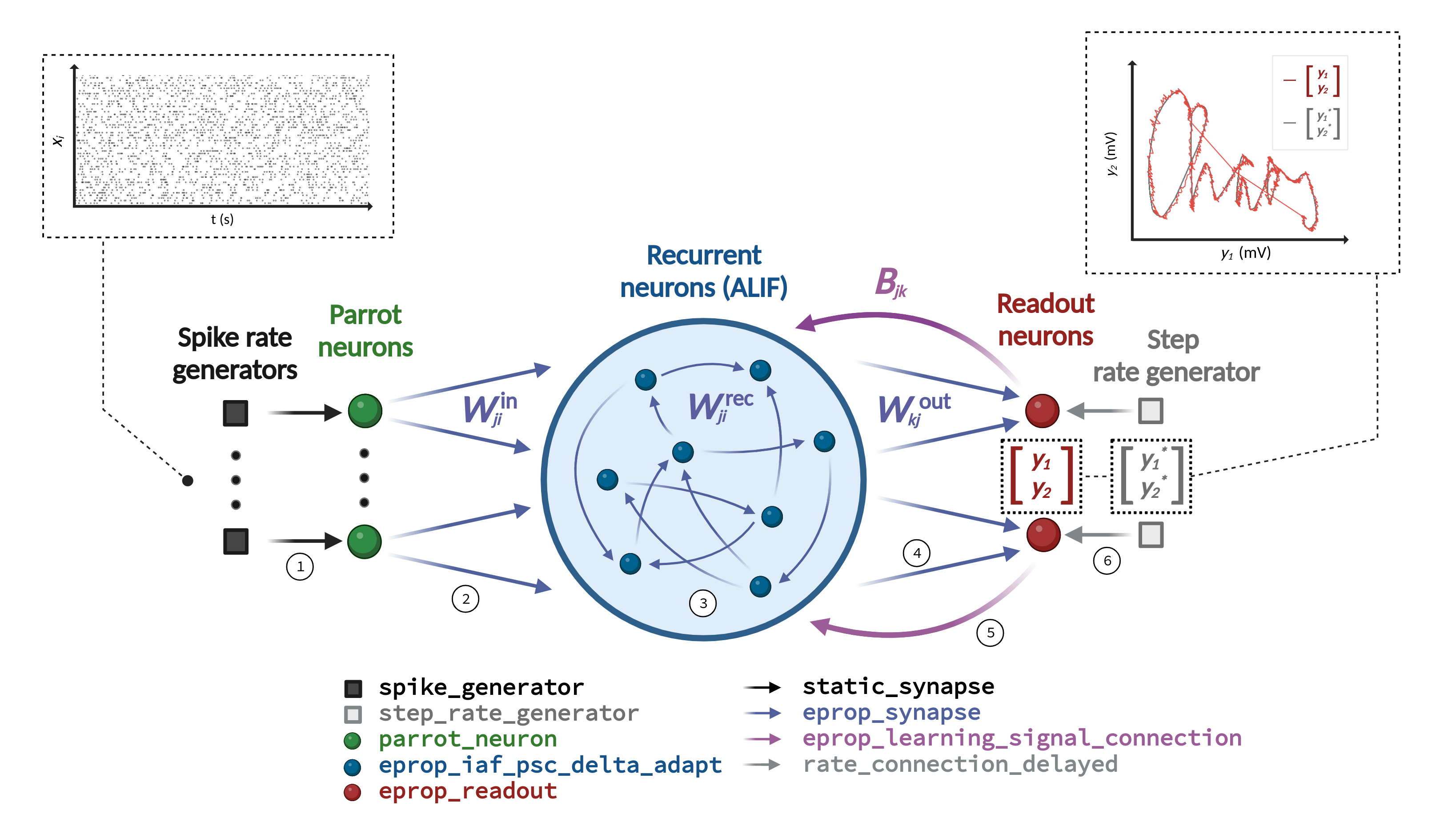
Learning in the neural network model is achieved by optimizing the connection weights with e-prop plasticity. This plasticity rule requires a specific network architecture depicted in Figure 1. The neural network model consists of a recurrent network that receives frozen noise input from Poisson generators and projects onto two readout neurons. Each individual readout signal denoted as \(y_k\) is compared with a corresponding target signal represented as \(y_k^*\). The network’s training error is assessed by employing a mean-squared error loss.

Details on the event-based NEST implementation of e-prop can be found in [3].

The development of this task and the hyper-parameter optimization were conducted by Agnes Korcsak-Gorzo and Charl Linssen, inspired by activities and feedback received at the CapoCaccia Workshop toward Neuromorphic Intelligence 2023.

References

[1] (1,2)

Bellec G, Scherr F, Subramoney F, Hajek E, Salaj D, Legenstein R, Maass W (2020). A solution to the learning dilemma for recurrent networks of spiking neurons. Nature Communications, 11:3625. https://doi.org/10.1038/s41467-020-17236-y

[2]

https://github.com/IGITUGraz/eligibility_propagation/blob/master/Figure_3_and_S7_e_prop_tutorials/tutorial_pattern_generation.py

[3]

Korcsak-Gorzo A, Stapmanns J, Espinoza Valverde JA, Dahmen D, van Albada SJ, Bolten M, Diesmann M. Event-based implementation of eligibility propagation (in preparation)

Import libraries

We begin by importing all libraries required for the simulation, analysis, and visualization.

import matplotlib as mpl
import matplotlib.pyplot as plt
import nest
import numpy as np
from cycler import cycler
from IPython.display import Image

Schematic of network architecture

This figure, identical to the one in the description, shows the required network architecture in the center, the input and output of the pattern generation task above, and lists of the required NEST device, neuron, and synapse models below. The connections that must be established are numbered 1 to 6.

try:
    Image(filename="./eprop_supervised_regression_schematic_handwriting.png")
except Exception:
    pass

Setup

Initialize random generator

We seed the numpy random generator, which will generate random initial weights as well as random input and output.

rng_seed = 1  # numpy random seed
np.random.seed(rng_seed)  # fix numpy random seed

Define timing of task

The task’s temporal structure is then defined, once as time steps and once as durations in milliseconds.

n_batch = 1  # batch size
n_iter = 5  # number of iterations, 5000 for good convergence

data_file_name = "chaos_handwriting.txt"  # name of file with task data
data = np.loadtxt(data_file_name)

steps = {
    "data_point": 8,  # time steps of one data point
}

steps["sequence"] = len(data) * steps["data_point"]  # time steps of one full sequence
steps["learning_window"] = steps["sequence"]  # time steps of window with non-zero learning signals
steps["task"] = n_iter * n_batch * steps["sequence"]  # time steps of task

steps.update(
    {
        "offset_gen": 1,  # offset since generator signals start from time step 1
        "delay_in_rec": 1,  # connection delay between input and recurrent neurons
        "delay_rec_out": 1,  # connection delay between recurrent and output neurons
        "delay_out_norm": 1,  # connection delay between output neurons for normalization
        "extension_sim": 1,  # extra time step to close right-open simulation time interval in Simulate()
    }
)

steps["delays"] = steps["delay_in_rec"] + steps["delay_rec_out"] + steps["delay_out_norm"]  # time steps of delays

steps["total_offset"] = steps["offset_gen"] + steps["delays"]  # time steps of total offset

steps["sim"] = steps["task"] + steps["total_offset"] + steps["extension_sim"]  # time steps of simulation

duration = {"step": 1.0}  # ms, temporal resolution of the simulation

duration.update({key: value * duration["step"] for key, value in steps.items()})  # ms, durations

Set up simulation

As last step of the setup, we reset the NEST kernel to remove all existing NEST simulation settings and objects and set some NEST kernel parameters, some of which are e-prop-related.

params_setup = {
    "eprop_learning_window": duration["learning_window"],
    "eprop_reset_neurons_on_update": True,  # if True, reset dynamic variables at start of each update interval
    "eprop_update_interval": duration["sequence"],  # ms, time interval for updating the synaptic weights
    "print_time": False,  # if True, print time progress bar during simulation, set False if run as code cell
    "resolution": duration["step"],
    "total_num_virtual_procs": 1,  # number of virtual processes, set in case of distributed computing
    "rng_seed": rng_seed,  # seed for NEST random generator
}

nest.ResetKernel()
nest.set(**params_setup)

Create neurons

We proceed by creating a certain number of input, recurrent, and readout neurons and setting their parameters. Additionally, we already create an input spike generator and an output target rate generator, which we will configure later.

n_in = 100  # number of input neurons
n_rec = 200  # number of recurrent neurons
n_out = 2  # number of readout neurons

tau_m_mean = 30.0  # ms, mean of membrane time constant distribution

params_nrn_rec = {
    "adapt_tau": 2000.0,  # ms, time constant of adaptive threshold
    "C_m": 250.0,  # pF, membrane capacitance - takes effect only if neurons get current input (here not the case)
    "c_reg": 150.0,  # firing rate regularization scaling
    "E_L": 0.0,  # mV, leak / resting membrane potential
    "f_target": 20.0,  # spikes/s, target firing rate for firing rate regularization
    "gamma": 0.3,  # scaling of the pseudo derivative
    "I_e": 0.0,  # pA, external current input
    "regular_spike_arrival": False,  # If True, input spikes arrive at end of time step, if False at beginning
    "surrogate_gradient_function": "piecewise_linear",  # surrogate gradient / pseudo-derivative function
    "t_ref": 0.0,  # ms, duration of refractory period
    "tau_m": nest.random.normal(mean=tau_m_mean, std=2.0),  # ms, membrane time constant
    "V_m": 0.0,  # mV, initial value of the membrane voltage
    "V_th": 0.03,  # mV, spike threshold membrane voltage
}

params_nrn_rec["adapt_beta"] = (
    1.7 * (1.0 - np.exp(-1 / params_nrn_rec["adapt_tau"])) / (1.0 - np.exp(-1.0 / tau_m_mean))
)  # prefactor of adaptive threshold

params_nrn_out = {
    "C_m": 1.0,
    "E_L": 0.0,
    "I_e": 0.0,
    "loss": "mean_squared_error",  # loss function
    "regular_spike_arrival": False,
    "tau_m": 50.0,
    "V_m": 0.0,
}

# Intermediate parrot neurons required between input spike generators and recurrent neurons,
# since devices cannot establish plastic synapses for technical reasons

gen_spk_in = nest.Create("spike_generator", n_in)
nrns_in = nest.Create("parrot_neuron", n_in)

# The suffix _bsshslm_2020 follows the NEST convention to indicate in the model name the paper
# that introduced it by the first letter of the authors' last names and the publication year.

nrns_rec = nest.Create("eprop_iaf_adapt_bsshslm_2020", n_rec, params_nrn_rec)
nrns_out = nest.Create("eprop_readout_bsshslm_2020", n_out, params_nrn_out)
gen_rate_target = nest.Create("step_rate_generator", n_out)

Create recorders

We also create recorders, which, while not required for the training, will allow us to track various dynamic variables of the neurons, spikes, and changes in synaptic weights. To save computing time and memory, the recorders, the recorded variables, neurons, and synapses can be limited to the ones relevant to the experiment, and the recording interval can be increased (see the documentation on the specific recorders). By default, recordings are stored in memory but can also be written to file.

n_record = 1  # number of neurons to record dynamic variables from - this script requires n_record >= 1
n_record_w = 3  # number of senders and targets to record weights from - this script requires n_record_w >=1

if n_record == 0 or n_record_w == 0:
    raise ValueError("n_record and n_record_w >= 1 required")

params_mm_rec = {
    "interval": duration["step"],  # interval between two recorded time points
    "record_from": [
        "V_m",
        "surrogate_gradient",
        "learning_signal",
        "V_th_adapt",
        "adaptation",
    ],  # dynamic variables to record
    "start": duration["offset_gen"] + duration["delay_in_rec"],  # start time of recording
    "stop": duration["offset_gen"] + duration["delay_in_rec"] + duration["task"],  # stop time of recording
}

params_mm_out = {
    "interval": duration["step"],
    "record_from": ["V_m", "readout_signal", "readout_signal_unnorm", "target_signal", "error_signal"],
    "start": duration["total_offset"],
    "stop": duration["total_offset"] + duration["task"],
}

params_wr = {
    "senders": nrns_in[:n_record_w] + nrns_rec[:n_record_w],  # limit senders to subsample weights to record
    "targets": nrns_rec[:n_record_w] + nrns_out,  # limit targets to subsample weights to record from
    "start": duration["total_offset"],
    "stop": duration["total_offset"] + duration["task"],
}

params_sr = {
    "start": duration["total_offset"],
    "stop": duration["total_offset"] + duration["task"],
}

mm_rec = nest.Create("multimeter", params_mm_rec)
mm_out = nest.Create("multimeter", params_mm_out)
sr = nest.Create("spike_recorder", params_sr)
wr = nest.Create("weight_recorder", params_wr)

nrns_rec_record = nrns_rec[:n_record]

Create connections

Now, we define the connectivity and set up the synaptic parameters, with the synaptic weights drawn from normal distributions. After these preparations, we establish the enumerated connections of the core network, as well as additional connections to the recorders.

params_conn_all_to_all = {"rule": "all_to_all", "allow_autapses": False}
params_conn_one_to_one = {"rule": "one_to_one"}

dtype_weights = np.float32  # data type of weights - for reproducing TF results set to np.float32
weights_in_rec = np.array(np.random.randn(n_in, n_rec).T / np.sqrt(n_in), dtype=dtype_weights)
weights_rec_rec = np.array(np.random.randn(n_rec, n_rec).T / np.sqrt(n_rec), dtype=dtype_weights)
np.fill_diagonal(weights_rec_rec, 0.0)  # since no autapses set corresponding weights to zero
weights_rec_out = np.array(np.random.randn(n_rec, n_out).T / np.sqrt(n_rec), dtype=dtype_weights)
weights_out_rec = np.array(np.random.randn(n_rec, n_out) / np.sqrt(n_rec), dtype=dtype_weights)

params_common_syn_eprop = {
    "optimizer": {
        "type": "adam",  # algorithm to optimize the weights
        "batch_size": n_batch,
        "beta_1": 0.9,  # exponential decay rate for 1st moment estimate of Adam optimizer
        "beta_2": 0.999,  # exponential decay rate for 2nd moment raw estimate of Adam optimizer
        "epsilon": 1e-8,  # small numerical stabilization constant of Adam optimizer
        "eta": 5e-3,  # learning rate
        "Wmin": -100.0,  # pA, minimal limit of the synaptic weights
        "Wmax": 100.0,  # pA, maximal limit of the synaptic weights
    },
    "average_gradient": False,  # if True, average the gradient over the learning window
    "weight_recorder": wr,
}

params_syn_base = {
    "synapse_model": "eprop_synapse_bsshslm_2020",
    "delay": duration["step"],  # ms, dendritic delay
    "tau_m_readout": params_nrn_out["tau_m"],  # ms, for technical reasons pass readout neuron membrane time constant
}

params_syn_in = params_syn_base.copy()
params_syn_in["weight"] = weights_in_rec  # pA, initial values for the synaptic weights

params_syn_rec = params_syn_base.copy()
params_syn_rec["weight"] = weights_rec_rec

params_syn_out = params_syn_base.copy()
params_syn_out["weight"] = weights_rec_out

params_syn_feedback = {
    "synapse_model": "eprop_learning_signal_connection_bsshslm_2020",
    "delay": duration["step"],
    "weight": weights_out_rec,
}

params_syn_rate_target = {
    "synapse_model": "rate_connection_delayed",
    "delay": duration["step"],
    "receptor_type": 2,  # receptor type over which readout neuron receives target signal
}

params_syn_static = {
    "synapse_model": "static_synapse",
    "delay": duration["step"],
}

params_init_optimizer = {
    "optimizer": {
        "m": 0.0,  # initial 1st moment estimate m of Adam optimizer
        "v": 0.0,  # initial 2nd moment raw estimate v of Adam optimizer
    }
}

nest.SetDefaults("eprop_synapse_bsshslm_2020", params_common_syn_eprop)

nest.Connect(gen_spk_in, nrns_in, params_conn_one_to_one, params_syn_static)  # connection 1
nest.Connect(nrns_in, nrns_rec, params_conn_all_to_all, params_syn_in)  # connection 2
nest.Connect(nrns_rec, nrns_rec, params_conn_all_to_all, params_syn_rec)  # connection 3
nest.Connect(nrns_rec, nrns_out, params_conn_all_to_all, params_syn_out)  # connection 4
nest.Connect(nrns_out, nrns_rec, params_conn_all_to_all, params_syn_feedback)  # connection 5
nest.Connect(gen_rate_target, nrns_out, params_conn_one_to_one, params_syn_rate_target)  # connection 6

nest.Connect(nrns_in + nrns_rec, sr, params_conn_all_to_all, params_syn_static)

nest.Connect(mm_rec, nrns_rec_record, params_conn_all_to_all, params_syn_static)
nest.Connect(mm_out, nrns_out, params_conn_all_to_all, params_syn_static)

# After creating the connections, we can individually initialize the optimizer's
# dynamic variables for single synapses (here exemplarily for two connections).

nest.GetConnections(nrns_rec[0], nrns_rec[1:3]).set([params_init_optimizer] * 2)

Create input

We generate some frozen Poisson spike noise of a fixed rate that is repeated in each iteration and feed these spike times to the previously created input spike generator. The network will use these spike times as a temporal backbone for encoding the target signal into its recurrent spiking activity.

input_spike_prob = 0.05  # spike probability of frozen input noise
dtype_in_spks = np.float32  # data type of input spikes - for reproducing TF results set to np.float32

input_spike_bools = (np.random.rand(steps["sequence"], n_in) < input_spike_prob).swapaxes(0, 1)
input_spike_bools[:, 0] = 0  # remove spikes in 0th time step of every sequence for technical reasons

sequence_starts = np.arange(0.0, duration["task"], duration["sequence"]) + duration["offset_gen"]
params_gen_spk_in = []
for input_spike_bool in input_spike_bools:
    input_spike_times = np.arange(0.0, duration["sequence"], duration["step"])[input_spike_bool]
    input_spike_times_all = [input_spike_times + start for start in sequence_starts]
    params_gen_spk_in.append({"spike_times": np.hstack(input_spike_times_all).astype(dtype_in_spks)})

nest.SetStatus(gen_spk_in, params_gen_spk_in)

Create output

Then, we load the x and y values of an image of the word “chaos” written by hand and construct a roughly two-second long target signal from it. This signal, like the input, is repeated for all iterations and fed into the rate generator that was previously created.

x_eval = np.arange(steps["sequence"]) / steps["data_point"]
x_data = np.arange(steps["sequence"] // steps["data_point"])

target_signal_list = []
for y_data in np.cumsum(data, axis=0).T:
    y_data /= np.max(np.abs(y_data))
    y_data -= np.mean(y_data)
    target_signal_list.append(np.interp(x_eval, x_data, y_data))

params_gen_rate_target = []

for target_signal in target_signal_list:
    params_gen_rate_target.append(
        {
            "amplitude_times": np.arange(0.0, duration["task"], duration["step"]) + duration["total_offset"],
            "amplitude_values": np.tile(target_signal, n_iter * n_batch),
        }
    )

nest.SetStatus(gen_rate_target, params_gen_rate_target)

Force final update

Synapses only get active, that is, the correct weight update calculated and applied, when they transmit a spike. To still be able to read out the correct weights at the end of the simulation, we force spiking of the presynaptic neuron and thus an update of all synapses, including those that have not transmitted a spike in the last update interval, by sending a strong spike to all neurons that form the presynaptic side of an eprop synapse. This step is required purely for technical reasons.

gen_spk_final_update = nest.Create("spike_generator", 1, {"spike_times": [duration["task"] + duration["delays"]]})

nest.Connect(gen_spk_final_update, nrns_in + nrns_rec, "all_to_all", {"weight": 1000.0})

Read out pre-training weights

Before we begin training, we read out the initial weight matrices so that we can eventually compare them to the optimized weights.

def get_weights(pop_pre, pop_post):
    conns = nest.GetConnections(pop_pre, pop_post).get(["source", "target", "weight"])
    conns["senders"] = np.array(conns["source"]) - np.min(conns["source"])
    conns["targets"] = np.array(conns["target"]) - np.min(conns["target"])

    conns["weight_matrix"] = np.zeros((len(pop_post), len(pop_pre)))
    conns["weight_matrix"][conns["targets"], conns["senders"]] = conns["weight"]
    return conns


weights_pre_train = {
    "in_rec": get_weights(nrns_in, nrns_rec),
    "rec_rec": get_weights(nrns_rec, nrns_rec),
    "rec_out": get_weights(nrns_rec, nrns_out),
}

Simulate

We train the network by simulating for a set simulation time, determined by the number of iterations and the batch size and the length of one sequence.

nest.Simulate(duration["sim"])

Read out post-training weights

After the training, we can read out the optimized final weights.

weights_post_train = {
    "in_rec": get_weights(nrns_in, nrns_rec),
    "rec_rec": get_weights(nrns_rec, nrns_rec),
    "rec_out": get_weights(nrns_rec, nrns_out),
}

Read out recorders

We can also retrieve the recorded history of the dynamic variables and weights, as well as detected spikes.

events_mm_rec = mm_rec.get("events")
events_mm_out = mm_out.get("events")
events_sr = sr.get("events")
events_wr = wr.get("events")

Evaluate training error

We evaluate the network’s training error by calculating a loss - in this case, the mean squared error between the integrated recurrent network activity and the target rate.

readout_signal = events_mm_out["readout_signal"]
target_signal = events_mm_out["target_signal"]
senders = events_mm_out["senders"]

loss_list = []
for sender in set(senders):
    idc = senders == sender
    error = (readout_signal[idc] - target_signal[idc]) ** 2
    loss_list.append(0.5 * np.add.reduceat(error, np.arange(0, steps["task"], steps["sequence"])))

loss = np.sum(loss_list, axis=0)

Plot results

Then, we plot a series of plots.

do_plotting = True  # if True, plot the results

if not do_plotting:
    exit()

colors = {
    "blue": "#2854c5ff",
    "red": "#e04b40ff",
    "white": "#ffffffff",
}

plt.rcParams.update(
    {
        "font.sans-serif": "Arial",
        "axes.spines.right": False,
        "axes.spines.top": False,
        "axes.prop_cycle": cycler(color=[colors["blue"], colors["red"]]),
    }
)

Plot pattern

First, we visualize the created pattern and plot the target for comparison. The outputs of the two readout neurons encode the horizontal and vertical coordinate of the pattern respectively.

fig, ax = plt.subplots()

ax.plot(
    readout_signal[senders == list(set(senders))[0]][-steps["sequence"] :],
    -readout_signal[senders == list(set(senders))[1]][-steps["sequence"] :],
    c=colors["red"],
    label="readout",
)

ax.plot(
    target_signal[senders == list(set(senders))[0]][-steps["sequence"] :],
    -target_signal[senders == list(set(senders))[1]][-steps["sequence"] :],
    c=colors["blue"],
    label="target",
)

ax.set_xlabel(r"$y_0$ and $y^*_0$")
ax.set_ylabel(r"$y_1$ and $y^*_1$")

ax.axis("equal")

fig.tight_layout()

Plot training error

We begin with a plot visualizing the training error of the network: the loss plotted against the iterations.

fig, ax = plt.subplots()

ax.plot(range(1, n_iter + 1), loss_list[0], label=r"$E_0$", alpha=0.8, c=colors["blue"], ls="--")
ax.plot(range(1, n_iter + 1), loss_list[1], label=r"$E_1$", alpha=0.8, c=colors["blue"], ls="dotted")
ax.plot(range(1, n_iter + 1), loss, label=r"$E$", c=colors["blue"])
ax.set_ylabel(r"$E = \frac{1}{2} \sum_{t,k} \left( y_k^t -y_k^{*,t}\right)^2$")
ax.set_xlabel("training iteration")
ax.set_xlim(1, n_iter)
ax.xaxis.get_major_locator().set_params(integer=True)
ax.legend(bbox_to_anchor=(1.01, 0.5), loc="center left")
fig.tight_layout()

Plot spikes and dynamic variables

This plotting routine shows how to plot all of the recorded dynamic variables and spikes across time. We take one snapshot in the first iteration and one snapshot at the end.

def plot_recordable(ax, events, recordable, ylabel, xlims):
    for sender in set(events["senders"]):
        idc_sender = events["senders"] == sender
        idc_times = (events["times"][idc_sender] > xlims[0]) & (events["times"][idc_sender] < xlims[1])
        ax.plot(events["times"][idc_sender][idc_times], events[recordable][idc_sender][idc_times], lw=0.5)
    ax.set_ylabel(ylabel)
    margin = np.abs(np.max(events[recordable]) - np.min(events[recordable])) * 0.1
    ax.set_ylim(np.min(events[recordable]) - margin, np.max(events[recordable]) + margin)


def plot_spikes(ax, events, nrns, ylabel, xlims):
    idc_times = (events["times"] > xlims[0]) & (events["times"] < xlims[1])
    idc_sender = np.isin(events["senders"][idc_times], nrns.tolist())
    senders_subset = events["senders"][idc_times][idc_sender]
    times_subset = events["times"][idc_times][idc_sender]

    ax.scatter(times_subset, senders_subset, s=0.1)
    ax.set_ylabel(ylabel)
    margin = np.abs(np.max(senders_subset) - np.min(senders_subset)) * 0.1
    ax.set_ylim(np.min(senders_subset) - margin, np.max(senders_subset) + margin)


for xlims in [(0, steps["sequence"]), (steps["task"] - steps["sequence"], steps["task"])]:
    fig, axs = plt.subplots(12, 1, sharex=True, figsize=(8, 12), gridspec_kw={"hspace": 0.4, "left": 0.2})

    plot_spikes(axs[0], events_sr, nrns_in, r"$z_i$" + "\n", xlims)
    plot_spikes(axs[1], events_sr, nrns_rec, r"$z_j$" + "\n", xlims)

    plot_spikes(axs[3], events_sr, nrns_rec, r"$z_j$" + "\n", xlims)

    plot_recordable(axs[4], events_mm_rec, "V_m", r"$v_j$" + "\n(mV)", xlims)
    plot_recordable(axs[5], events_mm_rec, "surrogate_gradient", r"$\psi_j$" + "\n", xlims)
    plot_recordable(axs[6], events_mm_rec, "V_th_adapt", r"$A_j$" + "\n(mV)", xlims)
    plot_recordable(axs[7], events_mm_rec, "learning_signal", r"$L_j$" + "\n(pA)", xlims)

    plot_recordable(axs[8], events_mm_out, "V_m", r"$v_k$" + "\n(mV)", xlims)
    plot_recordable(axs[9], events_mm_out, "target_signal", r"$y^*_k$" + "\n", xlims)
    plot_recordable(axs[10], events_mm_out, "readout_signal", r"$y_k$" + "\n", xlims)
    plot_recordable(axs[11], events_mm_out, "error_signal", r"$y_k-y^*_k$" + "\n", xlims)

    axs[-1].set_xlabel(r"$t$ (ms)")
    axs[-1].set_xlim(*xlims)

    fig.align_ylabels()

Plot weight time courses

Similarly, we can plot the weight histories. Note that the weight recorder, attached to the synapses, works differently than the other recorders. Since synapses only get activated when they transmit a spike, the weight recorder only records the weight in those moments. That is why the first weight registrations do not start in the first time step and we add the initial weights manually.

def plot_weight_time_course(ax, events, nrns_senders, nrns_targets, label, ylabel):
    for sender in nrns_senders.tolist():
        for target in nrns_targets.tolist():
            idc_syn = (events["senders"] == sender) & (events["targets"] == target)
            idc_syn_pre = (weights_pre_train[label]["source"] == sender) & (
                weights_pre_train[label]["target"] == target
            )

            times = [0.0] + events["times"][idc_syn].tolist()
            weights = [weights_pre_train[label]["weight"][idc_syn_pre]] + events["weights"][idc_syn].tolist()

            ax.step(times, weights, c=colors["blue"])
        ax.set_ylabel(ylabel)
        ax.set_ylim(-0.6, 0.6)


fig, axs = plt.subplots(3, 1, sharex=True, figsize=(3, 4))

plot_weight_time_course(axs[0], events_wr, nrns_in[:n_record_w], nrns_rec[:n_record_w], "in_rec", r"$W_\text{in}$ (pA)")
plot_weight_time_course(
    axs[1], events_wr, nrns_rec[:n_record_w], nrns_rec[:n_record_w], "rec_rec", r"$W_\text{rec}$ (pA)"
)
plot_weight_time_course(axs[2], events_wr, nrns_rec[:n_record_w], nrns_out, "rec_out", r"$W_\text{out}$ (pA)")

axs[-1].set_xlabel(r"$t$ (ms)")
axs[-1].set_xlim(0, steps["task"])

fig.align_ylabels()
fig.tight_layout()

Plot weight matrices

If one is not interested in the time course of the weights, it is possible to read out only the initial and final weights, which requires less computing time and memory than the weight recorder approach. Here, we plot the corresponding weight matrices before and after the optimization.

cmap = mpl.colors.LinearSegmentedColormap.from_list(
    "cmap", ((0.0, colors["blue"]), (0.5, colors["white"]), (1.0, colors["red"]))
)

fig, axs = plt.subplots(3, 2, sharex="col", sharey="row")

all_w_extrema = []

for k in weights_pre_train.keys():
    w_pre = weights_pre_train[k]["weight"]
    w_post = weights_post_train[k]["weight"]
    all_w_extrema.append([np.min(w_pre), np.max(w_pre), np.min(w_post), np.max(w_post)])

args = {"cmap": cmap, "vmin": np.min(all_w_extrema), "vmax": np.max(all_w_extrema)}

for i, weights in zip([0, 1], [weights_pre_train, weights_post_train]):
    axs[0, i].pcolormesh(weights["in_rec"]["weight_matrix"].T, **args)
    axs[1, i].pcolormesh(weights["rec_rec"]["weight_matrix"], **args)
    cmesh = axs[2, i].pcolormesh(weights["rec_out"]["weight_matrix"], **args)

    axs[2, i].set_xlabel("recurrent\nneurons")

axs[0, 0].set_ylabel("input\nneurons")
axs[1, 0].set_ylabel("recurrent\nneurons")
axs[2, 0].set_ylabel("readout\nneurons")
fig.align_ylabels(axs[:, 0])

axs[0, 0].text(0.5, 1.1, "pre-training", transform=axs[0, 0].transAxes, ha="center")
axs[0, 1].text(0.5, 1.1, "post-training", transform=axs[0, 1].transAxes, ha="center")

axs[2, 0].yaxis.get_major_locator().set_params(integer=True)

cbar = plt.colorbar(cmesh, cax=axs[1, 1].inset_axes([1.1, 0.2, 0.05, 0.8]), label="weight (pA)")

fig.tight_layout()

plt.show()