
Part 4: Spatially structured networks
Introduction
This section covers how to use NEST to construct structured networks. When you have worked through this material you will be able to:
Create populations of neurons with specific spatial locations
Define connectivity profiles between these types of populations
Connect populations using profiles
Visualize the connectivity
For more information on the usage of PyNEST, please see the other sections of this tutorial:
More advanced examples can be found at Example
Networks, or
have a look at the source directory of your NEST installation in the
subdirectory: pynest/examples/.
Incorporating structure in networks of point neurons
If we use biologically detailed models of a neuron, then it’s easy to understand and implement the concepts of spatial networks, as we already have dendritic arbors, axons, etc. which are the physical prerequisites for connectivity within the nervous system. However, we can still get a level of specificity using networks of point neurons.
Structure, both in the topological and everyday sense, can be thought of as a set of rules governing the location of objects and the connections between them. Within networks of point neurons, we can distinguish between three types of specificity:
Cell-type specificity – what sorts of cells are there?
Location specificity – where are the cells?
Projection specificity – which cells do they project to, and how?
In the previous sections, we saw that we can create deterministic or
randomly selected connections between networks using Connect(). Likewise, it is
also possible to use Create() and Connect() to create network
models that incorporate spatial location and spatial connectivity
profiles.
Note
For comprehensive documentation of spatial properties and connectivity, see the Spatially-structured networks.
Adding spatial information to populations
NEST allows us to create populations of nodes with a given spatial structure, connection profiles which specify how neurons are to be connected, and provides a high-level connection routine. We can thus create structured networks by designing the connection profiles to give the desired specificity for cell-type, location and projection.
The generation of structured networks is carried out in three steps, each of which will be explained in the subsequent sections in more detail:
Defining spatially distributed nodes, in which we assign the layout and types of the neurons within a layer of our network.
Defining connection specifications, where we specify the parameters for connecting we wish our connections to have. Each connection dictionary specifies the properties for one class of connection, and contains parameters that allow us to tune the profile. These are related to the location-dependent likelihood of choosing a target (
maskandp).Connecting nodes, in which we apply the connection specifications between nodes, equivalent to population-specificity. A spatially distributed node can be connected to itself.
Auxillary, in which we visualise the results of the above steps either by
nest.PrintNodes()or visualization functions and query the connections for further analysis.
Defining spatially distributed nodes
The code for defining nodes with spatial distributions follows this template:
import nest
positions = ...  # See below for how to define positions
s_nodes = nest.Create(node_model, positions=positions)
where positions will define the locations of the elements.
The node_model is the model type of the neuron, which can either be an
existing model in the NEST collection, or one that we’ve previously
defined using CopyModel().
We next have to decide whether the nodes should be placed in a grid-based or free (off-grid) fashion, which is equivalent to asking “can the elements of our network be regularly and evenly placed within a 2D/3D network, or do we need to tell them where they should be located?”.
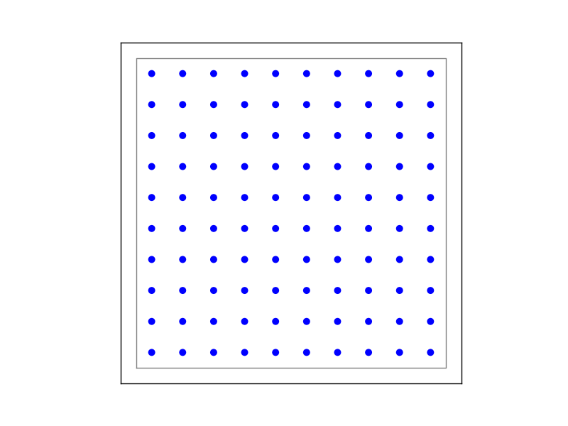
Figure 10 Example of on-grid, in which the neurons are positioned as grid.
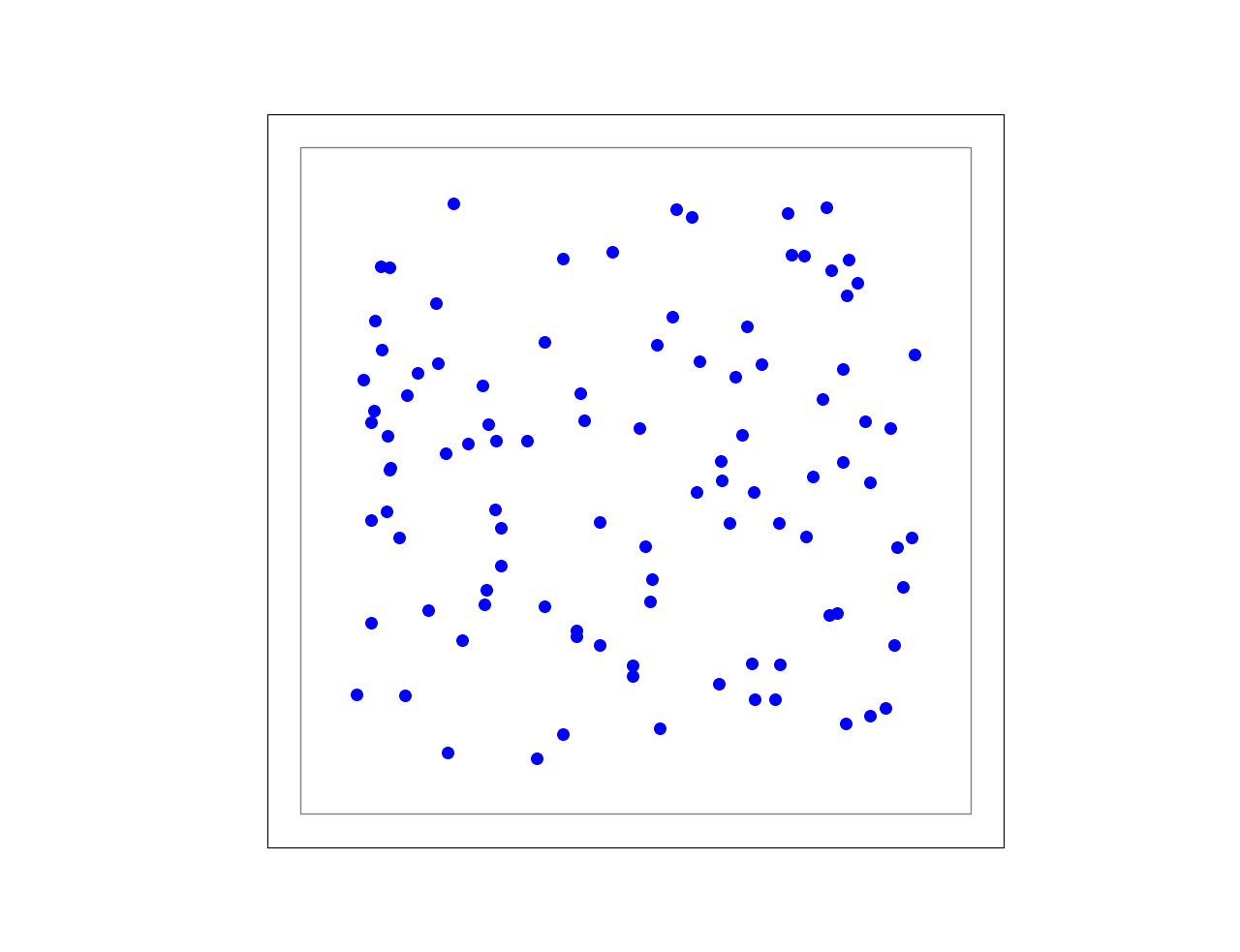
Figure 11 Example of a free layer, in which the neurons are positioned in a random uniform manner.
1 - On-grid
We have to explicitly specify the spacing of the grid with shape=[n, m], where m is the number of rows and n is the number of columns. It might be easier to think of shape as shape=[nx, ny], where nx is number of elements in x-direction and ny is number of directions in y-direction. The size (extent) of the layer has a default size of 1 x 1, but this you can also set yourself. The grid spacing i is determined from m, n and extent, and n x m elements are arranged symmetrically. Note that we can also specify a center to the grid, else the default offset is the origin.
The following snippet produces Figure 10:
positions = nest.spatial.grid(shape=[10, 10],  # the number of rows and column in this grid ...
                              extent=[2., 2.]  # the size of the grid in mm
                              )
nest.Create('iaf_psc_alpha', positions=positions)
2 - Off-grid
For more flexibility in how we distribute neurons, we can use free spatial placement. We then need to define a Parameter for the placement of the neurons, or we can define the positions of the neurons explicitly. Note that the extent is calculated from the positions of the nodes, but we can also explicitly specify it. See the Free layers section of the Spatially-structured networks for details.
The following snippet produces Figure 11:
positions = nest.spatial.free(
    nest.random.uniform(min=-0.5, max=0.5),  # using random positions in a uniform distribution
    num_dimensions=2  # have to specify number of dimensions
)
s_nodes = nest.Create('iaf_psc_alpha', 100, positions=positions)
Note that we have to specify the number of dimensions as we are using a random parameter for the positions. The number of dimensions can be either 2 or 3. If we specify extent or use an explicit array of positions, the number of dimensions is deduced by NEST. Also note that when creating the nodes, we specify the number of neurons to be created. This is not necessary when using an array of positions.
See the table of Spatially-structured specific NEST parameters in the Spatially-structured networks for a selection of NEST Parameters that can be used.
The following is an example of how to create off-grid nodes with a list of positions. It will create nodes with a grid+jitter structure.
xs = np.arange(-0.5, 0.501, 0.1)
poss = [[x, y] for y in xs for x in xs]
poss = [[p[0] + np.random.uniform(-0.03, 0.03), p[1] + np.random.uniform(-0.03, 0.03)] for p in poss]

positions = nest.spatial.free(poss)
s_nodes = nest.Create('iaf_psc_alpha', positions=positions)
Defining connection profiles
To define the types of connections that we want between populations of neurons, we specify a connection dictionary.
The connection dictionary for connecting populations with spatial
information is the same as when connecting populations without spatial
information, but with a few optional additions. If the connection rule
is one of pairwise_bernoulli, fixed_indegree or
fixed_outdegree, one may specify some additional parameters that
allows us to tune our connectivity profiles by tuning the likelihood of a
connection, the number of connections, or defining a subset of the nodes
to connect.
The Connections section in the Spatially-structured networks deals comprehensively with all the different possibilities, and it’s suggested that you look there for learning about the different constraints, as well as reading through the different examples listed there. Here are some representative examples for setting up a connectivity profile, and the following table lists the parameters that can be used.
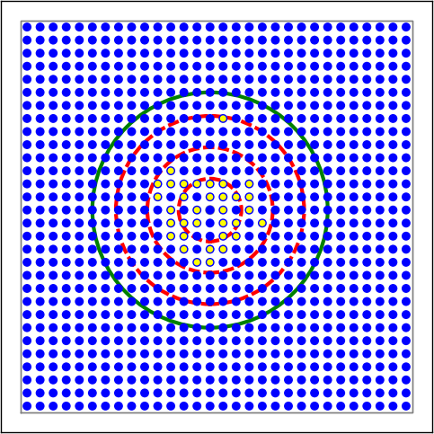
Figure 12 Examples of connectivity for each of the connectivity dictionaries mentioned in the following Python code snippet.
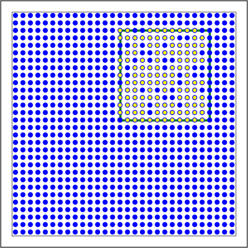
Figure 13 Examples of connectivity for each of the connectivity dictionaries mentioned in the following Python code snippet.
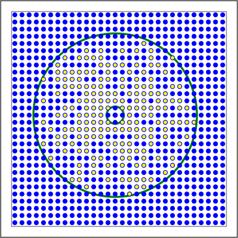
Figure 14 Examples of connectivity for each of the connectivity dictionaries mentioned in the following Python code snippet.
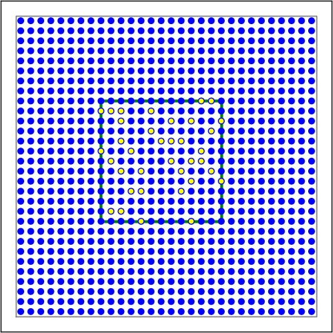
Figure 15 Examples of connectivity for each of the connectivity dictionaries mentioned in the following Python code snippet.
# Circular mask, distance-dependent connection probability with gaussian distribution
conn1 = {'rule': 'pairwise_bernoulli',
         'p': nest.spatial_distributions.gaussian(nest.spatial.distance, std=0.2),
         'mask': {'circular': {'radius': 0.75}},
         'allow_autapses': False
         }

# Rectangular mask with non-centered anchor, constant connection probability
conn2 = {'rule': 'pairwise_bernoulli',
         'p': 0.75,
         'mask': {'rectangular': {'lower_left': [-0.5, -0.5], 'upper_right': [0.5, 0.5]},
                 'anchor': [0.5, 0.5]},
         'allow_autapses': False
         }

# Donut mask, linear distance-dependent connection probability
conn3 = {'rule': 'pairwise_bernoulli',
         'p': 1.0 - 0.8 * nest.spatial.distance,
         'mask': {'doughnut': {'inner_radius': 0.1, 'outer_radius': 0.95}},
         }

# Rectangular mask, fixed outdegree, distance-dependent weights from a gaussian distribution,
# distance-dependent delays
conn4 = {'rule': 'fixed_outdegree',
         'outdegree': 40,
         'mask': {'rectangular': {'lower_left': [-0.5, -0.5], 'upper_right': [0.5, 0.5]}},
         'weight': nest.spatial_distributions.gaussian(
             J*nest.spatial.distance, std=0.25),
         'delay': 0.1 + 0.2 * nest.spatial.distance,
         'allow_autapses': False
         }
Parameter |
Description |
Possible values |
|---|---|---|
rule
|
Determines how nodes are selected when
connections are made.
|
Can be any connection rule, but for
spatial specific parameters has to
be one of the following:
pairwise_bernoulli,fixed_indegree,fixed_outdegree |
mask
|
Spatially selected subset of neurons considered
as (potential) targets
|
circular,
rectangular, elliptical,
doughnut, grid
|
p
|
Value or NEST Parameter that determines the
likelihood of a neuron being chosen as a target.
Can be distance-dependent.
|
constant,
NEST Parameter
|
weight
|
Distribution of weight values of connections.
Can be distance-dependent or -independent.
NB: this value overrides any value currently
used by synapse_model, and therefore unless
defined will default to 1.!
|
constant,
NEST Parameter
|
delay
|
Distribution of delay values for connections.
Can be distance-dependent or -independent.
NB: like weights, this value overrides any
value currently used by synapse_model!
|
constant,
NEST Parameter
|
synapse_model
|
Define the type of synapse model to be included.
|
any synapse model included in the
list returned by
nest.synapse_models |
use_on_source
|
Whether we want the mask and connection
probability to be applied to the source neurons
instead of the target neurons.
|
boolean
|
allow_multapses
|
Whether we want to have multiple connections
between the same source-target pair, or ensure
unique connections.
|
boolean
|
allow_autapses
|
Whether we want to allow a neuron to connect to
itself
|
boolean
|
Connecting spatially distributed nodes
Connecting spatially distributed nodes is the easiest step: having defined a source population, a
target population and a connection dictionary, we simply use
nest.Connect():
ex_pop = nest.Create('iaf_psc_alpha', positions=nest.spatial.grid(shape=[4, 5]))
in_pop = nest.Create('iaf_psc_alpha', positions=nest.spatial.grid(shape=[5, 4]))
conn_dict_ex = {'rule': 'pairwise_bernoulli',
                'p': 1.0,
                'mask': {'circular': {'radius': 0.5}}}
# And now we connect E->I
nest.Connect(ex_pop, in_pop, conn_dict_ex)
Note that we can use the same dictionary multiple times and connect to the same population:
# Extending the code from above ... we add a conn_dict for inhibitory neurons
conn_dict_in = {'rule': 'pairwise_bernoulli',
                'p': 1.0,
                'mask': {'circular': {'radius': 0.75}},
                'weight': -4.}
# And finish connecting the rest of the populations:
nest.Connect(ex_pop, ex_pop, conn_dict_ex)
nest.Connect(in_pop, in_pop, conn_dict_in)
nest.Connect(in_pop, ex_pop, conn_dict_in)
Visualising and querying the network structure
There are two main methods that we can use for checking that our network was built correctly:
nest.PrintNodes()which prints the node ID ranges and model names of the nodes in the network.
Create plots using the following functions:
nest.PlotLayer()nest.PlotTargets()nest.PlotSources()nest.PlotProbabilityParameter()
which allow us to generate the plots used with NUTM and this handout. See the Visualization functions section in our Spatially-structured networks for more details.
It may also be useful to look at the .spatial property of the
NodeCollection, which describes the spatial properties.
>>>  ex_pop.spatial
     {'center': (0.0, 0.0),
      'edge_wrap': False,
      'extent': (1.0, 1.0),
      'network_size': 20,
      'shape': (4, 5)}