Part 1: Neurons and simple neural networks
Introduction
In this section we cover the first steps in using PyNEST to simulate neuronal networks. When you have worked through this material, you will know how to:
start PyNEST
create neurons and stimulation or recording devices
query and set their parameters
connect them to each other or to devices
simulate the network
extract the data from recording devices
For more information on the usage of PyNEST, please see the other sections of this primer:
More advanced examples can be found at Example
Networks, or
have a look at at the source directory of your NEST installation in the
subdirectory: pynest/examples/.
PyNEST - an interface to the NEST simulator
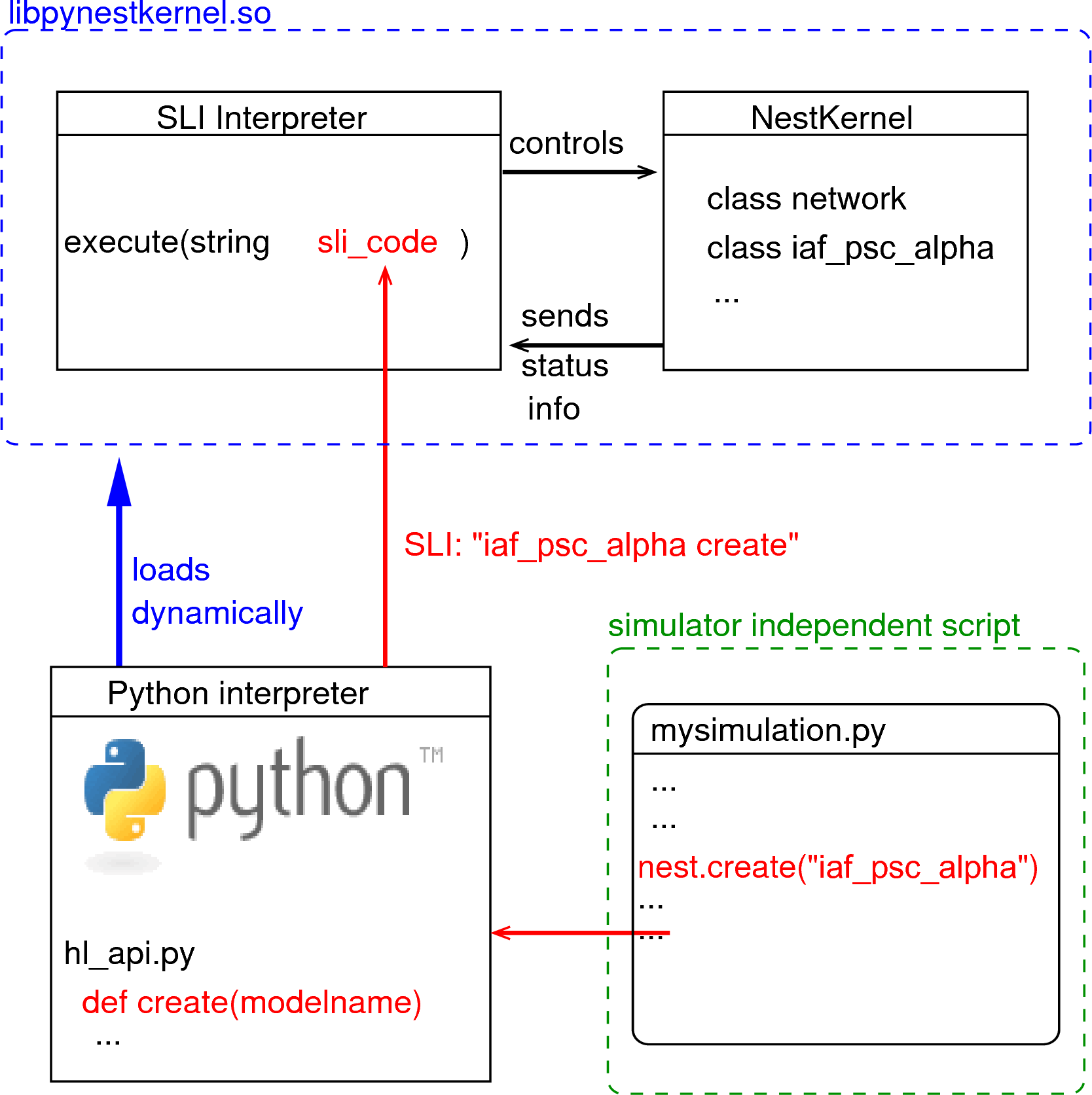
Figure 1 Python Interface Figure.
The Python interpreter imports NEST as a module and
dynamically loads the NEST simulator kernel (pynestkernel.so).
A simulation script of
the user (mysimulation.py) uses functions defined in this high-level
API. These functions generate code in SLI (Simulation Language
Interpreter), the native language of the interpreter of NEST. This
interpreter, in turn, controls the NEST simulation kernel.
The NEural Simulation Tool (NEST: www.nest-initiative.org) 1
is designed for the simulation of large heterogeneous networks of point
neurons. It is open source software released under the GPL licence. The
simulator comes with an interface to Python 2. Figure 1
illustrates the interaction between the user’s simulation script
(mysimulation.py) and the NEST simulator. Eppler et al. 3
contains a technically detailed description of the implementation of this
interface and parts of this text are based on this reference. The
simulation kernel is written in C++ to obtain the highest possible performance
for the simulation.
You can use PyNEST interactively from the Python prompt or from within IPython/Jupyter. This is very helpful when you are exploring PyNEST, trying to learn a new functionality or debugging a routine. Once out of the exploratory mode, you will find it saves a lot of time to write your simulations in text files. These can in turn be run from the command line or from the Python or ipython prompt.
Whether working interactively, semi-interactively, or purely executing scripts, the first thing that needs to happen is importing NEST’s functionality into the Python interpreter.
import nest
In case other Python packages are required, such as scikit-learn and SciPy, they need to be imported before importing NEST.
import sklearn
import scipy

import nest
As with every other module for Python, the available functions can be prompted for.
dir(nest)
If you want to obtain more information about a particular command, you
may use Python’s standard help system, which will return the help text
(docstring) explaining the use of this particular function. There is a
help system within NEST as well. You can open the help pages in a
browser using nest.helpdesk() and you can get the help page for a
particular NEST object (like a synapse or neuron model) using
nest.help('object').
Creating nodes
A neural network in NEST consists of two basic element types: nodes and connections. Nodes are either neurons, devices or sub-networks. Devices are used to stimulate neurons or to record from them. Nodes can be arranged with spatial structure to build networks distributed in space - we will get to this later in the course. For now we will work with the default network structure of NEST.
New nodes are created with the command Create(), which takes as arguments the model name of the
desired node type, and optionally the number of nodes to be created and
the initialising parameters. The function returns a NodeCollection of handles to
the new nodes, which you can assign to a variable for later use. A NodeCollection is a compact
representation of the node handles, which are integer numbers, called ids. Many PyNEST functions expect
or return a NodeCollection (see command overview). Thus, it is
easy to apply functions to large sets of nodes with a single function
call.
After having imported NEST and Matplotlib 4,
which we will use to display the results, we can start creating nodes.
As a first example, we will create a neuron of type
iaf_psc_alpha. This neuron is an integrate-and-fire neuron with
alpha-shaped postsynaptic currents. The function returns a NodeCollection of the
ids of all the created neurons, in this case only one, which we store in
a variable called neuron.
import matplotlib.pyplot as plt
import nest
neuron = nest.Create("iaf_psc_alpha")
We can now use the NodeCollection to access the properties of this neuron.
Properties of nodes in NEST are generally accessed via Python
dictionaries of key-value pairs of the form {key: value}. In order
to see which properties a neuron has, you may ask it for its status.
neuron.get()
This will print out the corresponding dictionary in the Python console.
Many of these properties are not relevant for the dynamics of the
neuron. To find out what the interesting properties are, look at the
documentation of the model through the helpdesk. If you already know
which properties you are interested in, you can specify a key, or a list
of keys, as an optional argument to get():
neuron.get("I_e")
neuron.get(["V_reset", "V_th"])
In the first case we query the value of the constant background current
I_e; the result is given as a floating point element. In the second
case, we query the values of the reset potential and threshold of the
neuron, and receive the result as a dictionary . If get() is
called on a NodeCollection with more than one element, the returned dictionary
will contain lists with the same number of elements as the number of nodes in
the NodeCollection. If get() is
called with a specific key on a NodeCollection with several elements, a list
the size of the NodeCollection will be returned.
To modify the properties in the dictionary, we use set(). In the
following example, the background current is set to 375.0pA, a value
causing the neuron to spike periodically.
neuron.set(I_e=375.0)
Note that we can set several properties at the same time by giving
multiple comma separated key:value pairs in a dictionary. Also be
aware that NEST is type sensitive - if a particular property is of type
double, then you do need to explicitly write the decimal point:
neuron.set({"I_e": 375})
will result in an error. This conveniently protects us from making integer division errors, which are hard to catch.
Another way of setting and getting parameters is to ask the NodeCollection directly
neuron.I_e = 376.0
neuron.I_e
Next we create a multimeter, a device we can use to record the
membrane voltage of a neuron over time. The property record_from
expects a list of the names of the variables we would like to
record. The variables exposed to the multimeter vary from model to
model. For a specific model, you can check the names of the exposed
variables by looking at the neuron’s property recordables.
multimeter = nest.Create("multimeter")
multimeter.set(record_from=["V_m"])
We now create a spike_recorder, another device that records the
spiking events produced by a neuron.
spikerecorder = nest.Create("spike_recorder")
A short note on naming: here we have called the neuron neuron, the
multimeter multimeter and so on. Of course, you can assign your
created nodes to any variable names you like, but the script is easier
to read if you choose names that reflect the concepts in your
simulation.
Connecting nodes with default connections
Now we know how to create individual nodes, we can start connecting them to form a small network.
nest.Connect(multimeter, neuron)
nest.Connect(neuron, spikerecorder)
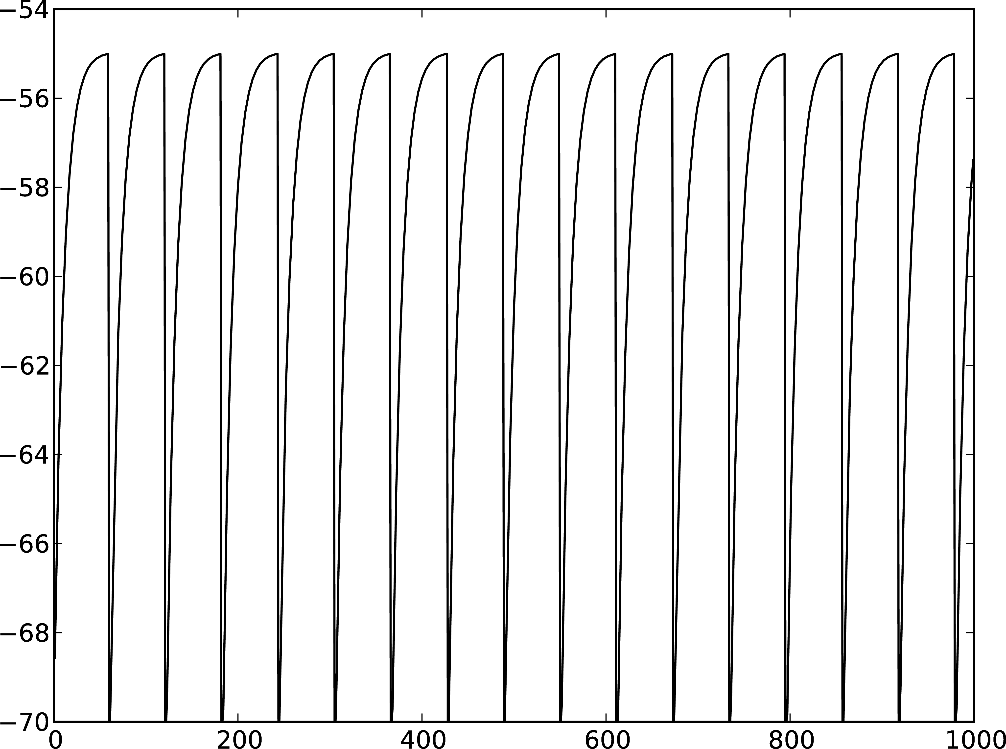
Figure 2 Membrane potential of integrate-and-fire neuron with constant input current.
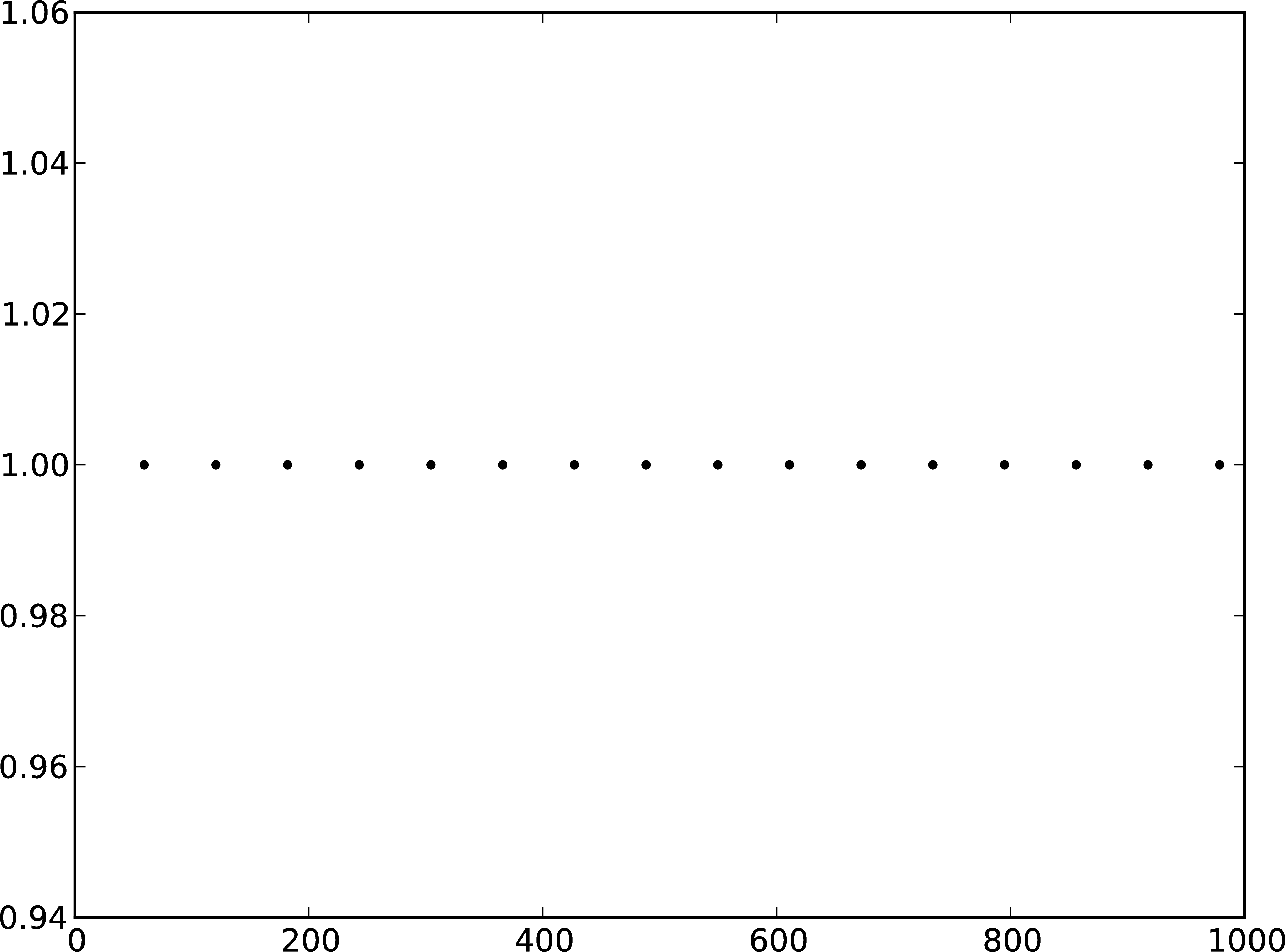
Figure 3 Spikes of the neuron.
The order in which the arguments to Connect() are specified reflects
the flow of events: if the neuron spikes, it sends an event to the spike
recorder. Conversely, the multimeter periodically sends requests to the
neuron to ask for its membrane potential at that point in time. This can
be regarded as a perfect electrode stuck into the neuron.
Now we have connected the network, we can start the simulation. We have to inform the simulation kernel how long the simulation is to run. Here we choose 1000ms.
nest.Simulate(1000.0)
Congratulations, you have just simulated your first network in NEST!
Extracting and plotting data from devices
After the simulation has finished, we can obtain the data recorded by the multimeter.
dmm = multimeter.get()
Vms = dmm["events"]["V_m"]
ts = dmm["events"]["times"]
In the first line, we obtain a dictionary with status parameters for the multimeter.
This dictionary contains an entry named events which holds the
recorded data. It is itself a dictionary with the entries V_m and
times, which we store separately in Vms and ts, in the
second and third line, respectively. If you are having trouble imagining
dictionaries of dictionaries and what you are extracting from where, try
first just printing dmm to the screen to give you a better
understanding of its structure, and then in the next step extract the
dictionary events, and so on.
Now we are ready to display the data in a figure. To this end, we make
use of matplotlib and the pyplot module.
import matplotlib.pyplot as plt
plt.figure(1)
plt.plot(ts, Vms)
The second line opens a figure (with the number 1), and the third line
actually produces the plot. You can’t see it yet because we have not
used plt.show(). Before we do that, we proceed analogously to
obtain and display the spikes from the spike recorder.
dSD = spikerecorder.get("events")
evs = dSD["senders"]
ts = dSD["times"]
plt.figure(2)
plt.plot(ts, evs, ".")
plt.show()
Here we extract the events more concisely by sending the parameter name to
get(). This extracts the dictionary element
with the key events rather than the whole status dictionary. The
output should look like Figure 2 and Figure 3.
If you want to execute this as a script, just paste all lines into a text
file named, say, one-neuron.py . You can then run it from the command
line by prefixing the file name with python, or from the Python or ipython
prompt, by prefixing it with Run().
It is possible to collect information of multiple neurons on a single multimeter. This does complicate retrieving the information: the data for each of the n neurons will be stored and returned in an interleaved fashion. Luckily Python provides us with a handy array operation to split the data easily: array slicing with a step (sometimes called stride). To explain this you have to adapt the model created in the previous part. Save your code under a new name, in the next section you will also work on this code. Create an extra neuron with the background current given a different value:
neuron2 = nest.Create("iaf_psc_alpha")
neuron2.set({"I_e": 370.0})
now connect this newly created neuron to the multimeter:
nest.Connect(multimeter, neuron2)
Run the simulation and plot the results, they will look incorrect. To
fix this you must plot the two neuron traces separately. Replace the
code that extracts the events from the multimeter with the following
lines.
plt.figure(2)
Vms1 = dmm["events"]["V_m"][::2] # start at index 0: till the end: each second entry
ts1 = dmm["events"]["times"][::2]
plt.plot(ts1, Vms1)
Vms2 = dmm["events"]["V_m"][1::2] # start at index 1: till the end: each second entry
ts2 = dmm["events"]["times"][1::2]
plt.plot(ts2, Vms2)
Additional information can be found at http://docs.scipy.org/doc/numpy-1.10.0/reference/arrays.indexing.html.
Connecting nodes with specific connections
A commonly used model of neural activity is the Poisson process. We now
adapt the previous example so that the neuron receives 2 Poisson spike
trains, one excitatory and the other inhibitory. Hence, we need a new
device, the poisson_generator. After creating the neurons, we create
these two generators and set their rates to 80000Hz and 15000Hz,
respectively.
noise_ex = nest.Create("poisson_generator")
noise_in = nest.Create("poisson_generator")
noise_ex.set(rate=80000.0)
noise_in.set(rate=15000.0)
Additionally, the constant input current should be set to 0:
neuron.set(I_e=0.0)
Each event of the excitatory generator should produce a postsynaptic
current of 1.2pA amplitude, an inhibitory event of -2.0pA. The
synaptic weights can be defined in a dictionary, which is passed to
the Connect() function using the keyword syn_spec
(synapse specifications). In general all parameters determining the
synapse can be specified in the synapse dictionary, such as
"weight", "delay", the synaptic model ("synapse_model")
and parameters specific to the synaptic model.
syn_dict_ex = {"weight": 1.2}
syn_dict_in = {"weight": -2.0}
nest.Connect(noise_ex, neuron, syn_spec=syn_dict_ex)
nest.Connect(noise_in, neuron, syn_spec=syn_dict_in)
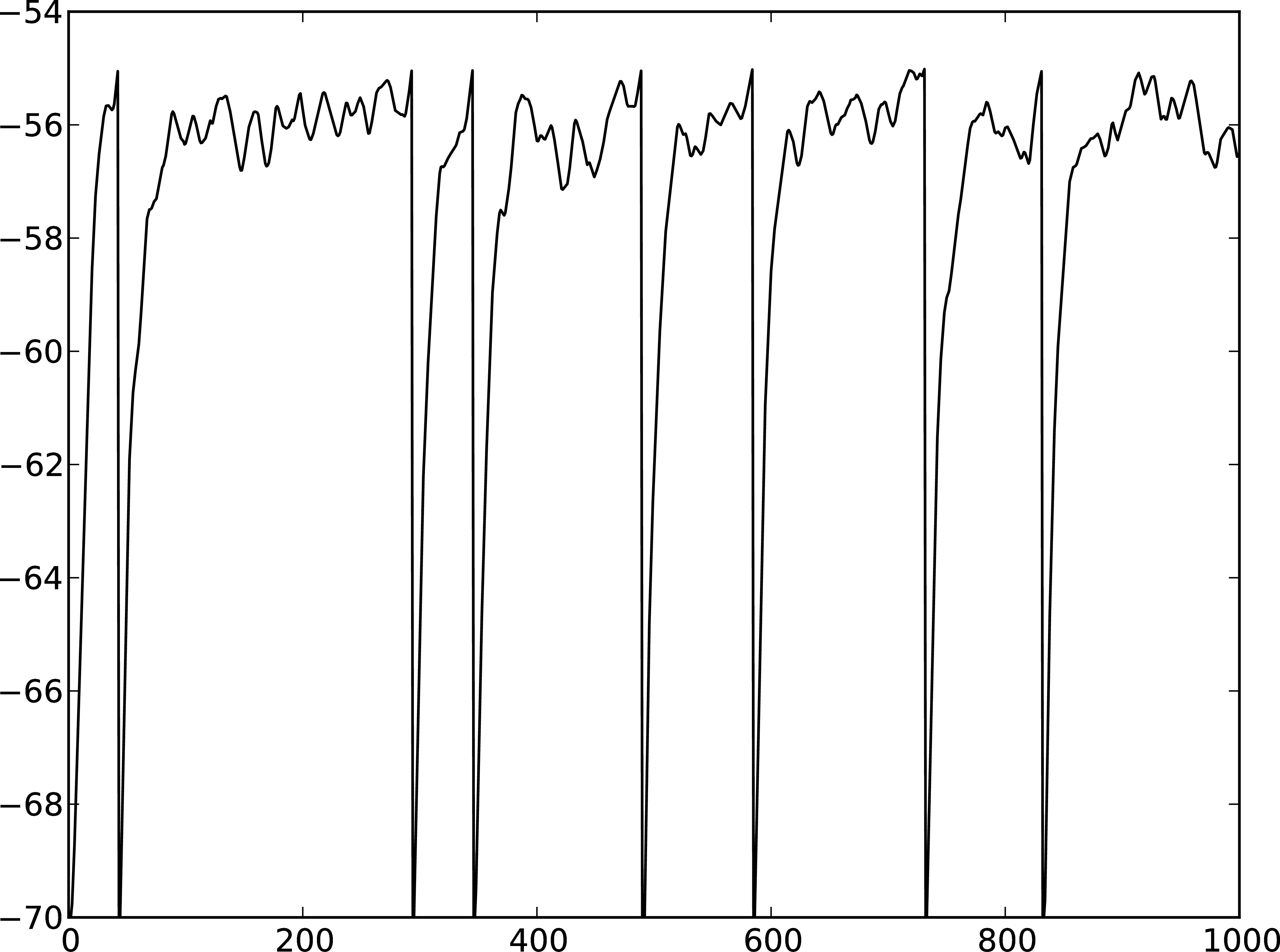
Figure 4 Membrane potential of integrate-and-fire neuron with Poisson noise as input.
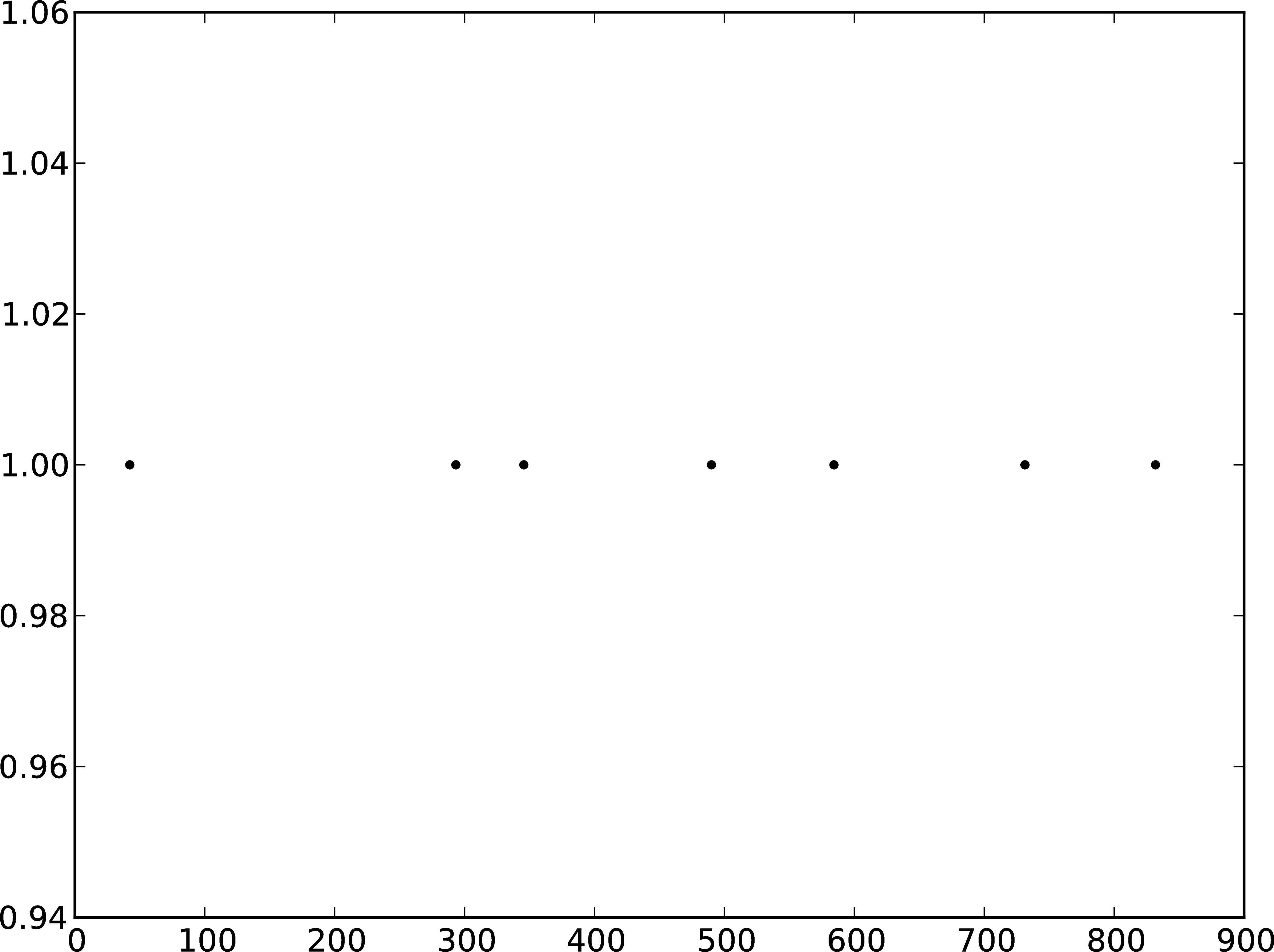
Figure 5 Spikes of the neuron with noise.
The rest of the code remains as before. You should see a membrane potential as in Figure 4 and Figure 5.
In the next part of the introduction (Part 2: Populations of neurons) we will look at more methods for connecting many neurons at once.
Two connected neurons
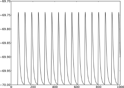
Figure 6 Postsynaptic potentials in neuron2 evoked by the spikes of neuron1
There is no additional magic involved in connecting neurons. To demonstrate this, we start from our original example of one neuron with a constant input current, and add a second neuron.
import nest
neuron1 = nest.Create("iaf_psc_alpha")
neuron1.set(I_e=376.0)
neuron2 = nest.Create("iaf_psc_alpha")
multimeter = nest.Create("multimeter")
multimeter.set(record_from=["V_m"])
We now connect neuron1 to neuron2, and record the membrane
potential from neuron2 so we can observe the postsynaptic potentials
caused by the spikes of neuron1.
nest.Connect(neuron1, neuron2, syn_spec = {"weight":20.0})
nest.Connect(multimeter, neuron2)
Here the default delay of 1ms was used. If the delay is specified in addition to the weight, the following shortcut is available:
nest.Connect(neuron1, neuron2, syn_spec={"weight":20.0, "delay":1.0})
If you simulate the network and plot the membrane potential as before,
you should then see the postsynaptic potentials of neuron2 evoked by
the spikes of neuron1 as in Figure 6.
Command overview
These are the functions we introduced for the examples in this handout; the following sections of this introduction will add more.
Getting information about NEST
See the Getting Help Section
Nodes
Create(model, n=1, params=None)Create
ninstances of typemodel. Parameters for the new nodes can be given asparams, which can be any of the following:A dictionary with either single values or lists of size n. The single values will be applied to all nodes, while the lists will be distributed across the nodes. Both single values and lists can be given at the same time.
A list with n dictionaries, one dictionary for each node.
If omitted, the
model’s defaults are used.
get(*params, **kwargs)Return a dictionary with parameter values for the NodeCollection it is called on. If
paramsis a single string, a list of values is returned instead.paramsmay also be a list of strings, in which case the returned dictionary contains lists of requested values.
set(params=None, **kwargs)Set the parameters on the NodeCollection to
params, which may be a single dictionary (with lists or single values as parameters), or a list of dictionaries of the same size as the NodeCollection. Ifkwargsis given, it has to be names and values of an attribute as keyword=argument pairs. The values can be single values or list of the same size as the NodeCollection.
Connections
This is an abbreviated version of the documentation for the Connect()
function, please see NEST’s online help for the full version and
Connection Management for an introduction
and examples.
Connect(pre, post, conn_spec=None, syn_spec=None, return_synapsecollection=False)Connect pre neurons to post neurons. Neurons in pre and post are connected using the specified connectivity (
"all_to_all"by default) and synapse type ("static_synapse"by default). Details depend on the connectivity rule.pre- presynaptic neurons, given as a NodeCollection of node IDspost- presynaptic neurons, given as a NodeCollection of node IDsconn_spec- name or dictionary specifying connectivity rule, see belowsyn_spec- name or dictionary specifying synapses, see below.
Connectivity
Connectivity is either specified as a string containing the name of a
connectivity rule (default: "all_to_all") or as a dictionary
specifying the rule and rule-specific parameters (e.g. "indegree"),
which must be given. In addition switches allowing self-connections
("allow_autapses", default: True) and multiple connections between a
pair of neurons ("allow_multapses", default: True) can be contained in
the dictionary.
Synapse
The synapse model and its properties can be inserted either as a
string naming a synapse model (see nest.synapse_models for all
available models) or as a dictionary. If no synapse model is
specified, the default model "static_synapse" will be used.
Available keys in the synapse dictionary are "synapse_model",
"weight", "delay", "receptor_type", as well as parameters
specific to the chosen synapse model. All parameters are optional and
if not specified will use the default values determined by the current
synapse model. "synapse_model" determines the synapse type, taken
from pre-defined synapse types in NEST or manually specified synapses
created via CopyModel(). All other parameters can be
scalars or distributions. In the case of scalar parameters, all keys
take doubles except for "receptor_type" which has to be
initialized with an integer. Distributed parameters are initialized
with a Parameter with distribution-specific arguments (such as
"mean" and "std").
Simulation control
Simulate(t)Simulate the network for
tmilliseconds.
References
- 1
Gewaltig MO. and Diesmann M. 2007. NEural Simulation Tool. 2(4):1430.
- 2
Python Software Foundation. The Python programming language, 2008. http://www.python.org.
- 3
Eppler JM et al. 2009 PyNEST: A convenient interface to the NEST simulator. 2:12. 10.3389/neuro.11.012.2008.
- 4
Hunter JD. 2007 Matplotlib: A 2d graphics environment. 9(3):90–95.