IAF neurons singularity

This notebook describes how NEST handles the singularities appearing in the ODE’s of integrate-and-fire model neurons with alpha- or exponentially-shaped current, when the membrane and the synaptic time-constants are identical.

import sympy as sp
sp.init_printing(use_latex=True)
from sympy.matrices import zeros
tau_m, tau_s, C, h = sp.symbols('tau_m, tau_s, C, h')

For alpha-shaped currents we have:

A = sp.Matrix([[-1/tau_s,0,0],[1,-1/tau_s,0],[0,1/C,-1/tau_m]])

Non-singular case (\(\tau_m\neq \tau_s\))

The propagator is:

PA = sp.simplify(sp.exp(A*h))
PA

$\displaystyle \left[\begin{matrix}e^{- \frac{h}{\tau_{s}}} & 0 & 0\\h e^{- \frac{h}{\tau_{s}}} & e^{- \frac{h}{\tau_{s}}} & 0\\\frac{\tau_{m} \tau_{s} \left(- h \left(\tau_{m} - \tau_{s}\right) e^{\frac{h \left(\tau_{m} + \tau_{s}\right)}{\tau_{m} \tau_{s}}} + \tau_{m} \tau_{s} e^{\frac{2 h}{\tau_{s}}} - \tau_{m} \tau_{s} e^{\frac{h \left(\tau_{m} + \tau_{s}\right)}{\tau_{m} \tau_{s}}}\right) e^{- \frac{h \left(2 \tau_{m} + \tau_{s}\right)}{\tau_{m} \tau_{s}}}}{C \left(\tau_{m} - \tau_{s}\right)^{2}} & \frac{\tau_{m} \tau_{s} \left(- e^{\frac{h}{\tau_{m}}} + e^{\frac{h}{\tau_{s}}}\right) e^{- \frac{h \left(\tau_{m} + \tau_{s}\right)}{\tau_{m} \tau_{s}}}}{C \left(\tau_{m} - \tau_{s}\right)} & e^{- \frac{h}{\tau_{m}}}\end{matrix}\right]$

Note that the entry in the third line and the second column \(A_{32}\) would also appear in the propagator matrix in case of an exponentially shaped current

Singular case (\(\tau_m = \tau_s\))

We have

As = sp.Matrix([[-1/tau_m,0,0],[1,-1/tau_m,0],[0,1/C,-1/tau_m]])
As

$\displaystyle \left[\begin{matrix}- \frac{1}{\tau_{m}} & 0 & 0\\1 & - \frac{1}{\tau_{m}} & 0\\0 & \frac{1}{C} & - \frac{1}{\tau_{m}}\end{matrix}\right]$

The propagator is

PAs = sp.simplify(sp.exp(As*h))
PAs

$\displaystyle \left[\begin{matrix}e^{- \frac{h}{\tau_{m}}} & 0 & 0\\h e^{- \frac{h}{\tau_{m}}} & e^{- \frac{h}{\tau_{m}}} & 0\\\frac{h^{2} e^{- \frac{h}{\tau_{m}}}}{2 C} & \frac{h e^{- \frac{h}{\tau_{m}}}}{C} & e^{- \frac{h}{\tau_{m}}}\end{matrix}\right]$

Numeric stability of propagator elements

For the lines \(\tau_s\rightarrow\tau_m\) the entry \(PA_{32}\) becomes numerically unstable, since denominator and enumerator go to zero.

1. We show that \(PAs_{32}\) is the limit of \(PA_{32}(\tau_s)\) for \(\tau_s\rightarrow\tau_m\).:

PA_32 = PA.row(2).col(1)[0]
sp.limit(PA_32, tau_s, tau_m)

$\displaystyle \frac{h e^{- \frac{h}{\tau_{m}}}}{C}$

2. The Taylor-series up to the second order of the function \(PA_{32}(\tau_s)\) is:

PA_32_series = PA_32.series(x=tau_s,x0=tau_m,n=2)
PA_32_series

$\displaystyle \frac{h e^{- \frac{h}{\tau_{m}}}}{C} + \frac{h^{2} \left(- \tau_{m} + \tau_{s}\right) e^{- \frac{h}{\tau_{m}}}}{2 C \tau_{m}^{2}} + O\left(\left(- \tau_{m} + \tau_{s}\right)^{2}; \tau_{s}\rightarrow \tau_{m}\right)$

Therefore we have

\(T(PA_{32}(\tau_s,\tau_m))=PAs_{32}+PA_{32}^{lin}+O(2)\) where \(PA_{32}^{lin}=h^2(-\tau_m + \tau_s)*exp(-h/\tau_m)/(2C\tau_m^2)\)

3. We define

\(dev:=|PA_{32}-PAs_{32}|\)

We also define \(PA_{32}^{real}\) which is the correct value of P32 without misscalculation (instability).

In the following we assume \(0<|\tau_s-\tau_m|<0.1\). We consider two different cases

a) When \(dev \geq 2|PA_{32}^{lin}|\) we do not trust the numeric evaluation of \(PA_{32}\), since it strongly deviates from the first order correction. In this case the error we make is

\(|PAs_{32}-PA_{32}^{real}|\approx |P_{32}^{lin}|\)

b) When \(dev \le |2PA_{32}^{lin}|\) we trust the numeric evaluation of \(PA_{32}\). In this case the maximal error occurs when \(dev\approx 2 PA_{32}^{lin}\) due to numeric instabilities. The order of the error is again

\(|PAs_{32}-PA_{32}^{real}|\approx |P_{32}^{lin}|\)

The entry \(A_{31}\) is numerically unstable, too and we treat it analogously.

Tests and examples

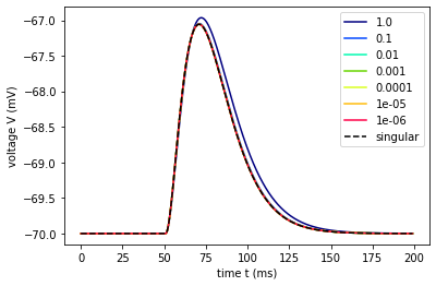
We will now show that the stability criterion explained above leads to a reasonable behavior for \(\tau_s\rightarrow\tau_m\)

import nest
import numpy as np
import pylab as pl

Neuron, simulation and plotting parameters

taum = 10.
C_m = 250.
# array of distances between tau_m and tau_ex
epsilon_array = np.hstack(([0.],10.**(np.arange(-6.,1.,1.))))[::-1]
dt = 0.1
fig = pl.figure(1)
NUM_COLORS = len(epsilon_array)
cmap = pl.get_cmap('gist_ncar')
maxVs = []

<Figure size 432x288 with 0 Axes>

Loop through epsilon array

for i,epsilon in enumerate(epsilon_array):
    nest.ResetKernel() # reset simulation kernel
    nest.SetKernelStatus({'resolution':dt})

    # Current based alpha neuron
    neuron = nest.Create('iaf_psc_alpha')
    neuron.set(C_m=C_m, tau_m=taum, t_ref=0., V_reset=-70., V_th=1e32,
               tau_syn_ex=taum+epsilon, tau_syn_in=taum+epsilon, I_e=0.)

    # create a spike generator
    spikegenerator_ex = nest.Create('spike_generator')
    spikegenerator_ex.spike_times = [50.]

    # create a voltmeter
    vm = nest.Create('voltmeter', params={'interval':dt})

    ## connect spike generator and voltmeter to the neuron
    nest.Connect(spikegenerator_ex, neuron, 'all_to_all', {'weight':100.})
    nest.Connect(vm, neuron)

    # run simulation for 200ms
    nest.Simulate(200.)

    # read out recording time and voltage from voltmeter
    times = vm.get('events','times')
    voltage = vm.get('events', 'V_m')

    # store maximum value of voltage trace in array
    maxVs.append(np.max(voltage))

    # plot voltage trace
    if epsilon == 0.:
        pl.plot(times,voltage,'--',color='black',label='singular')
    else:
        pl.plot(times,voltage,color = cmap(1.*i/NUM_COLORS),label=str(epsilon))

pl.legend()
pl.xlabel('time t (ms)')
pl.ylabel('voltage V (mV)')

Text(0, 0.5, 'voltage V (mV)')

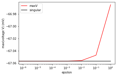
Show maximum values of voltage traces

fig = pl.figure(2)
pl.semilogx(epsilon_array,maxVs,color='red',label='maxV')
#show singular solution as horizontal line
pl.semilogx(epsilon_array,np.ones(len(epsilon_array))*maxVs[-1],color='black',label='singular')
pl.xlabel('epsilon')
pl.ylabel('max(voltage V) (mV)')
pl.legend()

<matplotlib.legend.Legend at 0x7f68764a5750>

pl.show()

The maximum of the voltage traces show that the non-singular case nicely converges to the singular one and no numeric instabilities occur.