
Siegert neuron integration
Alexander van Meegen, 2020-12-03
This notebook describes how NEST handles the numerical integration of the ‘Siegert’ function.
For an alternative approach, which was implemented in NEST before, see Appendix A.1 in (Hahne et al., 2017). The current approach seems to be faster and more stable, in particular in the noise-free limit.
Let’s start with some imports:
[1]:
import numpy as np
from scipy.special import erf, erfcx
import matplotlib.pyplot as plt
Introduction
We want to determine the firing rate of an integrate-and-fire neuron with exponentially decaying post–synaptic currents driven by a mean input \(\mu\) and white noise of strength \(\sigma\). For small synaptic time constant \(\tau_{\mathrm{s}}\) compared to the membrane time constant \(\tau_{\mathrm{m}}\), the firing rate is given by the ‘Siegert’ (Fourcaud and Brunel, 2002)
with the refractory period \(\tau_{\mathrm{ref}}\) and the integral
involving the shifted and scaled threshold voltage \(\tilde{V}_{\mathrm{th}}=\frac{V_{\mathrm{th}}-\mu}{\sigma}+\frac{\alpha}{2}\sqrt{\frac{\tau_{\mathrm{s}}}{\tau_{\mathrm{m}}}}\), the shifted and scaled reset voltage \(\tilde{V}_{\mathrm{r}}=\frac{V_{\mathrm{r}}-\mu}{\sigma}+\frac{\alpha}{2}\sqrt{\frac{\tau_{\mathrm{s}}}{\tau_{\mathrm{m}}}}\), and the constant \(\alpha=\sqrt{2}\left|\zeta(1/2)\right|\) where \(\zeta(x)\) denotes the Riemann zeta function.
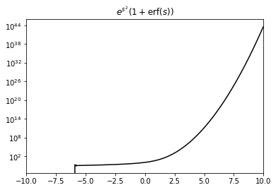
Numerically, the integral in \(I(\tilde{V}_{\mathrm{th}},\tilde{V}_{\mathrm{r}})\) is problematic due to the interplay of \(e^{s^{2}}\) and \(\mathrm{erf}(s)\) in the integrand. Already for moderate values of \(s\), it causes numerical problems (note the order of magnitude):
[2]:
s = np.linspace(-10, 10, 1001)
plt.plot(s, np.exp(s**2) * (1 + erf(s)), c="black")
plt.xlim(s[0], s[-1])
plt.yscale("log")
plt.title(r"$e^{s^{2}}(1+\mathrm{erf}(s))$")
plt.show()
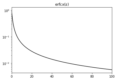
The main trick here is to use the scaled complementary error function
to extract the leading exponential contribution. For positive \(s\), we have \(0\le\mathrm{erfcx}(s)\le1\), i.e. the exponential contribution is in the prefactor \(e^{-s^{2}}\) which nicely cancels with the \(e^{s^{2}}\) in the integrand. In the following, we separate three cases according to the sign of \(\tilde{V}_{\mathrm{th}}\) and \(\tilde{V}_{\mathrm{r}}\) because for a negative arguments, the integrand simplifies to \(e^{s^{2}}(1+\mathrm{erf}(-s))=\mathrm{erfcx}(s)\). Eventually, only integrals of \(\mathrm{erfcx}(s)\) for positive \(s\ge0\) need to be solved numerically which are certainly better behaved:
[3]:
s = np.linspace(0, 100, 1001)
plt.plot(s, erfcx(s), c="black")
plt.xlim(s[0], s[-1])
plt.yscale("log")
plt.title(r"$\mathrm{erfcx}(s)$")
plt.show()
Mathematical Reformulation
Strong Inhibition
We have to consider three different cases; let us start with strong inhibitory input such that \(0<\tilde{V}_{\mathrm{r}}<\tilde{V}_{\mathrm{th}}\) or equivalently \(\mu<V_{\mathrm{r}}+\frac{\alpha}{2}\sigma\sqrt{\frac{\tau_{\mathrm{s}}}{\tau_{\mathrm{m}}}}\). In this regime, the error function in the integrand is positive. Expressing it in terms of \(\mathrm{erfcx}(s)\), we get
The first integral can be solved in terms of the Dawson function \(D(s)\), which is bound between \(\pm1\) and conveniently implemented in GSL; the second integral gives a small correction which has to be evaluated numerically. We get
We extract the leading contribution \(e^{\tilde{V}_{\mathrm{th}}^{2}}\) from the denominator and arrive at
as a numerically safe expression for \(0<\tilde{V}_{\mathrm{r}}<\tilde{V}_{\mathrm{th}}\). Extracting \(e^{\tilde{V}_{\mathrm{th}}^{2}}\) from the denominator reduces the latter to \(2\tau_{\mathrm{m}}\sqrt{\pi}D(\tilde{V}_{\mathrm{th}})\) and exponentially small correction terms because \(\tilde{V}_{\mathrm{r}}<\tilde{V}_{\mathrm{th}}\), thereby preventing overflow.
Strong Excitation
Now let us consider the case of strong excitatory input such that \(\tilde{V}_{\mathrm{r}}<\tilde{V}_{\mathrm{th}}<0\) or \(\mu>V_{\mathrm{th}}+\frac{\alpha}{2}\sigma\sqrt{\frac{\tau_{\mathrm{s}}}{\tau_{\mathrm{m}}}}\). In this regime, we can change variables \(s\to-s\) to make the domain of integration positive again. Using \(\mathrm{erf}(-s)=-\mathrm{erf}(s)\) as well as \(\mathrm{erfcx}(s)\), we get
In particular, there is no exponential contribution involved in this regime. Thus, we get
as a numerically safe expression for \(\tilde{V}_{\mathrm{r}}<\tilde{V}_{\mathrm{th}}<0\).
Intermediate Regime
In the intermediate regime, we have \(\tilde{V}_{\mathrm{r}}\le0\le\tilde{V}_{\mathrm{th}}\) or \(V_{\mathrm{r}}+\frac{\alpha}{2}\sigma\sqrt{\frac{\tau_{\mathrm{s}}}{\tau_{\mathrm{m}}}}\le\mu\le V_{\mathrm{th}}+\frac{\alpha}{2}\sigma\sqrt{\frac{\tau_{\mathrm{s}}}{\tau_{\mathrm{m}}}}\). Thus, we split the integral at zero and use the previous steps for the respective parts to get
Note that the sign of the second integral depends on whether \(\left|\tilde{V}_{\mathrm{r}}\right|>\tilde{V}_{\mathrm{th}}\) (+) or not (-). Again, we extract the leading contribution \(e^{\tilde{V}_{\mathrm{th}}^{2}}\) from the denominator and arrive at
as a numerically safe expressions for \(\tilde{V}_{\mathrm{r}}\le0\le\tilde{V}_{\mathrm{th}}\).
Noise-free Limit
Even the noise-free limit \(\sigma\ll\mu\), where the implementation from (Hahne et al., 2017) eventually breaks, works flawlessly. In this limit, \(\left|\tilde{V}_{\mathrm{th}}\right|\gg1\) as long as \(\mu\neq V_{\mathrm{th}}\); thus, we get both in the ‘strong inhibition’ and in the ‘itermediate’ regime \(\phi(\mu,\sigma)\sim e^{-\tilde{V}_{\mathrm{th}}^{2}}\approx0\) for \(\tilde{V}_{\mathrm{th}}\ge0\). Accordingly, the only interesting case is the ‘strong excitation’ regime \(\tilde{V}_{\mathrm{r}}<\tilde{V}_{\mathrm{th}}<0\). Since also \(\left|\tilde{V}_{\mathrm{r}}\right|\gg1\), the integrand \(\mathrm{erfcx}(s)\) is only evaluated at \(s\gg1\). Using the only the first term of the asymptotic expansion
leads to the analytically solvable integral
Inserting this into \(\phi(\mu,\sigma)\) and using \(\tilde{V}_{\mathrm{th}}\approx\frac{V_{\mathrm{th}}-\mu}{\sigma}, \tilde{V}_{\mathrm{r}}\approx\frac{V_{\mathrm{r}}-\mu}{\sigma}\) yields
as it should. Thus, as long as the numerical solution of the integral \(\frac{1}{\sqrt{\pi}}\int_{|\tilde{V}_{\mathrm{th}}|}^{|\tilde{V}_{\mathrm{r}}|}\frac{1}{s}ds\) is precise, the deterministic limit is also numerically safe.
Relevance of Noise-free Limit
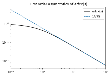
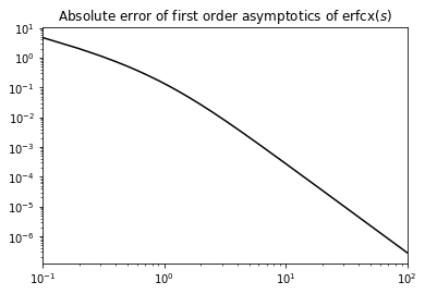
Let us briefly estimate for which values the noise-free limit becomes relevant. We have \(\left|\tilde{V}_{\mathrm{r}}\right|>\left|\tilde{V}_{\mathrm{th}}\right|\gg1\), thus the integrand \(\mathrm{erfcx}(s)\) is only evaluated for arguments \(s>\left|\tilde{V}_{\mathrm{th}}\right|\gg1\). Looking at the difference between \(\mathrm{erfcx}(s)\) and the first order asymptotics shown below, we see that the absolute difference to the asymptotics is only \(O(10^{-7})\) for moderate values \(\left|\tilde{V}_{\mathrm{th}}\right|\approx O(100)\). Since we saw above that the noise free limit is equivalent to the first order asymptotics, we can conclude that it is certainly relevant for \(\left|\tilde{V}_{\mathrm{th}}\right|\approx\frac{\mu-V_{\mathrm{th}}}{\sigma}\approx O(100)\); e.g. for \(\mu-V_{\mathrm{th}}\approx10\)mV a noise strength of \(\sigma\approx0.1\)mV corresponds to the noise-free limit.
[4]:
s = np.linspace(0.1, 100, 1000)
plt.plot(s, erfcx(s), c="black", label=r"$\mathrm{erfcx}(s)$")
plt.plot(s, 1 / (np.sqrt(np.pi) * s), ls="--", label=r"$1/\sqrt{\pi}s$")
plt.xlim(s[0], s[-1])
plt.xscale("log")
plt.yscale("log")
plt.legend()
plt.title(r"First order asymptotics of $\mathrm{erfcx}(s)$")
plt.show()
[5]:
s = np.linspace(0.1, 100, 1000)
plt.plot(s, 1 / (np.sqrt(np.pi) * s) - erfcx(s), c="black")
plt.xlim(s[0], s[-1])
plt.xscale("log")
plt.yscale("log")
plt.title(r"Absolute error of first order asymptotics of $\mathrm{erfcx}(s)$")
plt.show()
License
This file is part of NEST. Copyright (C) 2004 The NEST Initiative
NEST is free software: you can redistribute it and/or modify it under the terms of the GNU General Public License as published by the Free Software Foundation, either version 2 of the License, or (at your option) any later version.
NEST is distributed in the hope that it will be useful, but WITHOUT ANY WARRANTY; without even the implied warranty of MERCHANTABILITY or FITNESS FOR A PARTICULAR PURPOSE. See the GNU General Public License for more details.